Crypto Real Time Inference
These models run on device in your browser.
Crypto Real Time Inference
Overview
The aim of this application is to leverage historical cryptocurrency price data and cutting-edge machine learning algorithms to serve inferences about a cryptocurrency's future price points within a 1 hour window, in real time.
This was my first time working with time series data, and here we worked with raw time series datapoints that are served as OHLC ("open", "high", "low", "close") "candles". At a high level, I've chosen to think of a given cryptocurrency as a complex system (read: chaotic system), emergent as a phenomenon of large N interactions between groups of humans. Inherently, this is a social system.
In this framework, a "candle" is a measurement of a cryptocurrency's state at a given moment in time - and by measuring state at a series of time points we can see how the system's state evolves over time. The raw dataset itself (consisting of multiple candles) is a function that maps empirically measured states to time points. At a fundamental level, the same concepts can be applied to any physical system composed of a large number of interacting variables - which means this is a very challenging problem!
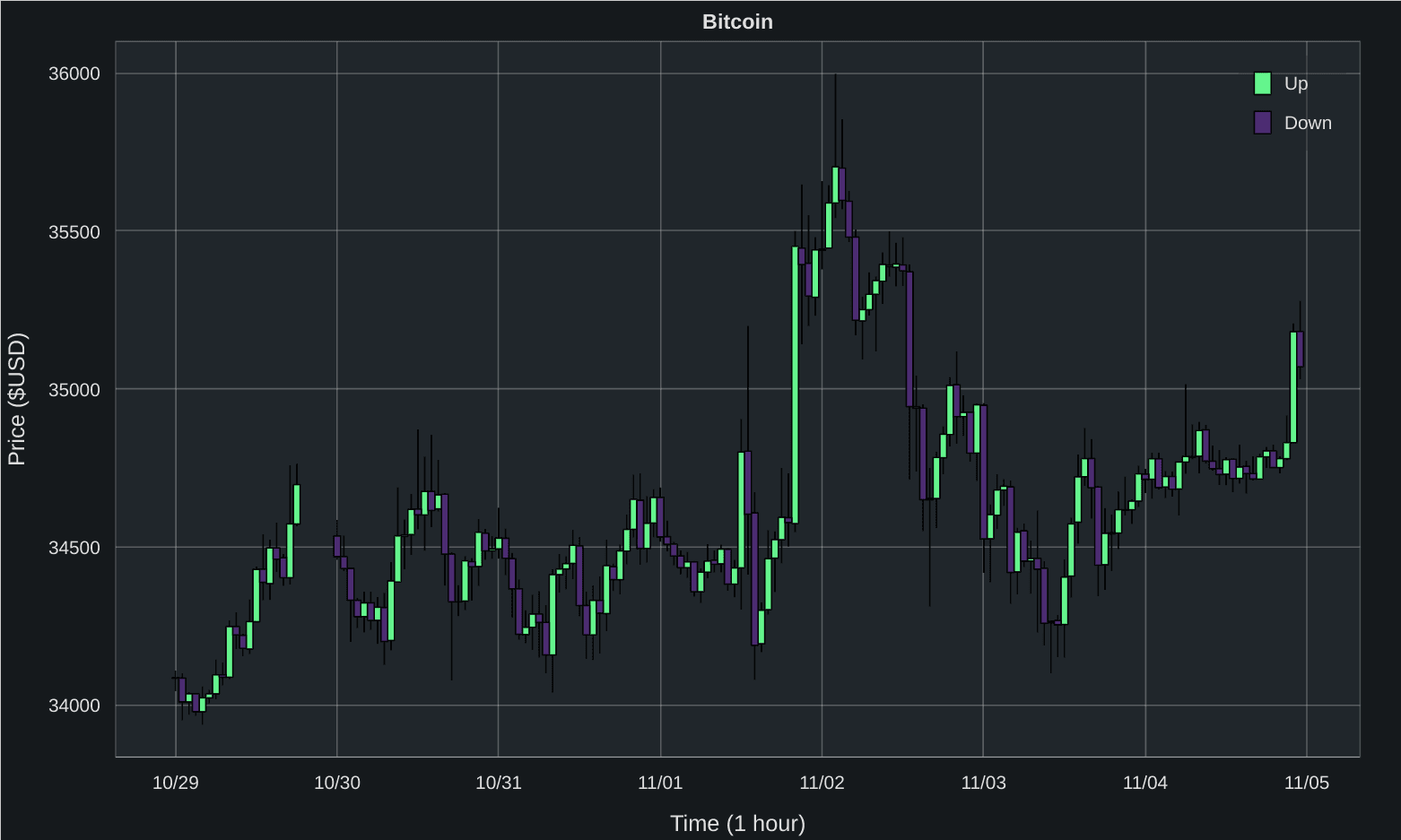
The visualization above is a snapshot of raw candle data used in this project. Cryptocurrency candles are pulled from Coinbase using their public API.
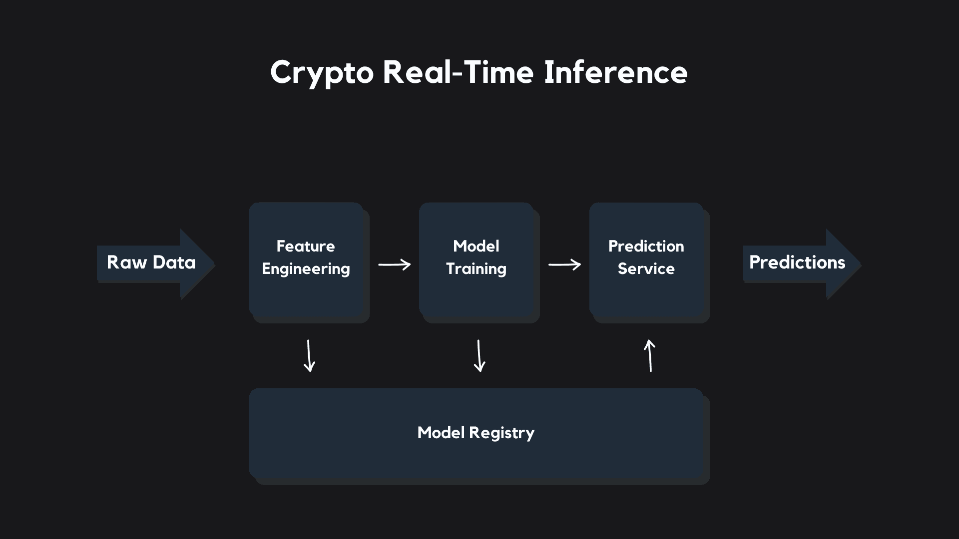
The application consists of eight components:
- Continuous Integration Pipeline: for source code integration
- Data Engineering Pipeline: that pulls raw cryptocurrency OHLC ("open", "high", "low", "close") candle data for a given cryptocurrency from Coinbase
- Feature Engineering Pipeline: that builds supervised-machine-learning-ready datasets from this raw data
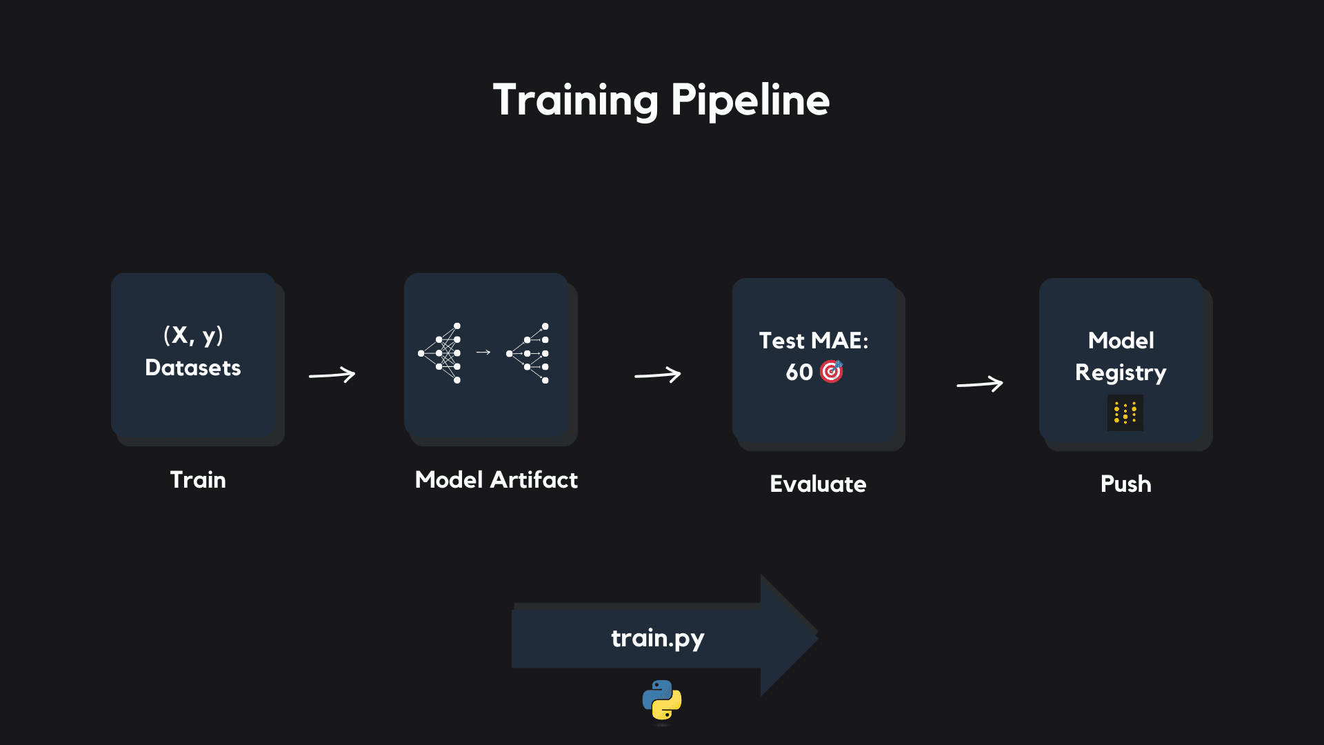
- Training Pipeline: that trains both machine learning and deep learning models, evaluates them, and pushes them up to our model registry
- Prediction Service: that serves model predictions using FastAPI
- Continuous Delivery Pipeline: that pulls our models from the registry, concurrently builds the prediction service into two Docker images (targeting x86_64 and arm64 chip architectures), and pushes them to Docker Hub
- Continuous Deployment Pipeline: with a web server written in Go that listens for webhooks from Docker Hub and deploys our prediction service onto a Raspberry Pi
- Frontend: built with Next.js, which you're using to view this
This project natively makes predictions for both Bitcoin and Ethereum pricepoints, though the source code supports any cryptocurrency that has publically available data.
Feature Engineering
Features are the variables (or information) that we give to machine learning models in order for them to make predictions.
Feature engineering is the process of extracting meaningful information from raw data that describes or encodes the process we are measuring, with the aim of improving our supervised machine learning algorithm's ability to make accurate predictions. Feature engineering plays a very key role in this project.
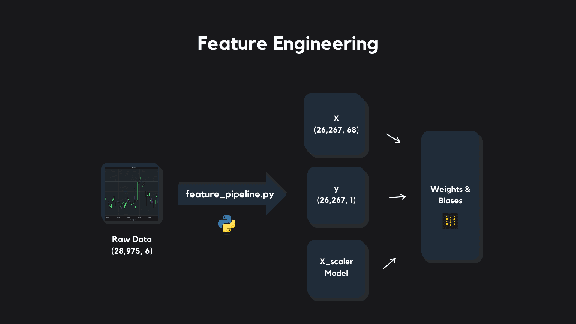
The raw OHLC ("open", "high", "low", "close") candle data is not fit for supervised machine learning modeling as is when we pull it down from Coinbase - it must be processed into a set of predictive features (an "X" dataset) and a target variable ("y" dataset) that we can train a model to make predictions with.
The preprocessing and feature engineering steps taken can be broken down as:
- Set "time" as the index and sort the dataset upfront by this index before lag features are generated
- Generate "Lag" X features ("price_i_hour_ago" and "volume_i_hour_ago" for past 24 hours) and y target ("target_price_next_hour")
- Compute window features for price and volume (moving average, moving standard deviation of past 24 hours)
- Calculate technical indicators (price percentage return, RSI)
- Split the full preprocessed dataset into an X features dataset and a y target dataset
- Fit a scaler model to the X data
- Version preprocessed datasets and X scaler model in model registry
At the end of this process we have an X features dataset that contains 68 features and a y target dataset that contains our prediction target that we can use to train supervised machine learning models.
Modeling
You can think of our feature engineering process as transforming the raw dataset of OHLC candles, which constitutes a 6-dimensional geometric space, into a 68-dimensional geometric space. Each candle which was once a 6-dimensional point is now a 68-dimensional point in this new space.
In this sense, during model development we are training models to map 68-dimensional points in our feature space to 1-dimensional points in our target space.
This application has infrastructure that supports both machine learning and deep learning modeling for cryptocurrency price predictions.
Machine Learning
The two machine learning algorithms I chose to explore here are the Lasso Regressor and Light Gradient Boosted Machine Regressor (LGBMRegressor) models.
Lasso Regressor
A Lasso Regressor is a variation of linear regression that incorporates a regularization term called L1 regularization, which is also known as the "Lasso" (Least Absolute Shrinkage and Selection Operator). The Lasso Regressor is designed to prevent overfitting and to perform feature selection by encouraging some of the model's coefficients to be exactly zero.
This means that a Lasso Regressor can automatically identify and exclude less important features, meaning that our resulting model is as simple as it can be given we want it to have the most predictive power possible.
My personal preference is always to reach for simple regression models first - not only do they serve as good baselines in your work if you end up requiring more complex modeling, they often perform quite well with some informed feature engineering choices or customization.
Light Gradient Boosted Machine Regressor
A Light Gradient Boosted Machine (LightGBM) is a powerful machine learning algorithm designed to be fast and memory-efficient. LightGBM is a gradient boosting framework, which means it builds a predictive model by combining the predictions of multiple weaker models, typically decision trees - these are also known as ensemble methods.
Ensemble methods are powerful, and often very successful in complex datasets.
The LGBMRegressor boasted a fast training time, but it did not appear to be suited for time series data. Ultimately I decided to move onto neural network modeling.
Deep Learning
The two deep learning algorithms I chose to implement here are the Convolutional Neural Network (CNN) and Long-Short Term Memory (LSTM) Neural Network models.
My original intuition was that a LSTM Neural Network would perform well, but I found that it was both slow and cumbersome and ill-suited for our features.
CNNs are typically used for image analysis tasks, but it turned out to be a great model to adapt for analyzing time series data.
CNNs use convolutional layers as their core building blocks. These layers consist of small filters (also known as kernels or receptive fields) that slide over the input feature vector.
The filters are responsible for capturing various local patterns in the data, such as edges, textures, and other low-level features in a typical image example. Here, local patterns in our cryptocurrency data would be relationships between previous price points and other information I calculated during feature engineering.
During the convolution operation, each filter scans the input vector and computes the element-wise dot product between the filter and the "local region" of the vector (meaning neighboring variables). This process generates a feature map for each filter.
A technique called pooling reduces the sizes of the computed feature maps, and once the feature maps have been extracted and pruned they are fed into a series of fully connected layers which perform traditional neural network operations.
A key hyperparameter I selected during experimentation was to use a kernel size of 4, meaning that the CNN scans the input vector 4 variables at a time. Using a 1-dimensional convolutional layer, this effectively allowed the model to discover patterns in price and volume changes over the past 24 hours, which I layed out sequentially within each feature vector.
Convolutional Neural Network Architecture
Neural network models were built using TensorFlow. With some experimenting I found that the Adam optimizer worked best. A learning rate of α = 0.001 was used. The CNN architecture I selected was:
- InputLayer((n_features, 1))
- Conv1D(256, kernel_size=4)
- Flatten()
- Dense(128, activation="relu")
- Activation("relu")
- Dense(128, activation="linear")
- Activation("relu")
- Dense(1, activation="linear")
Initial testing was run for a maximum of 20 epochs. After architecture selection and hyperparameter tuning, we used the best models saved from 300 epochs of training.
Experimental Results
A battery of experiments were run testing the Lasso Regressor, Light Gradient Boosted Machine Regressor (LGBMRegressor), Long Short-Term Memory (LSTM) Neural Network, and Convolution Neural Network (CNN) models respectively.
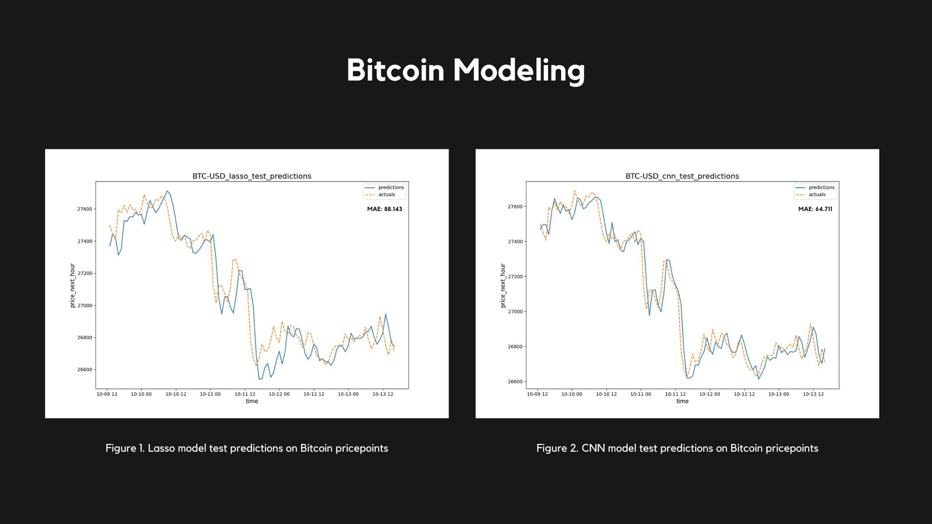
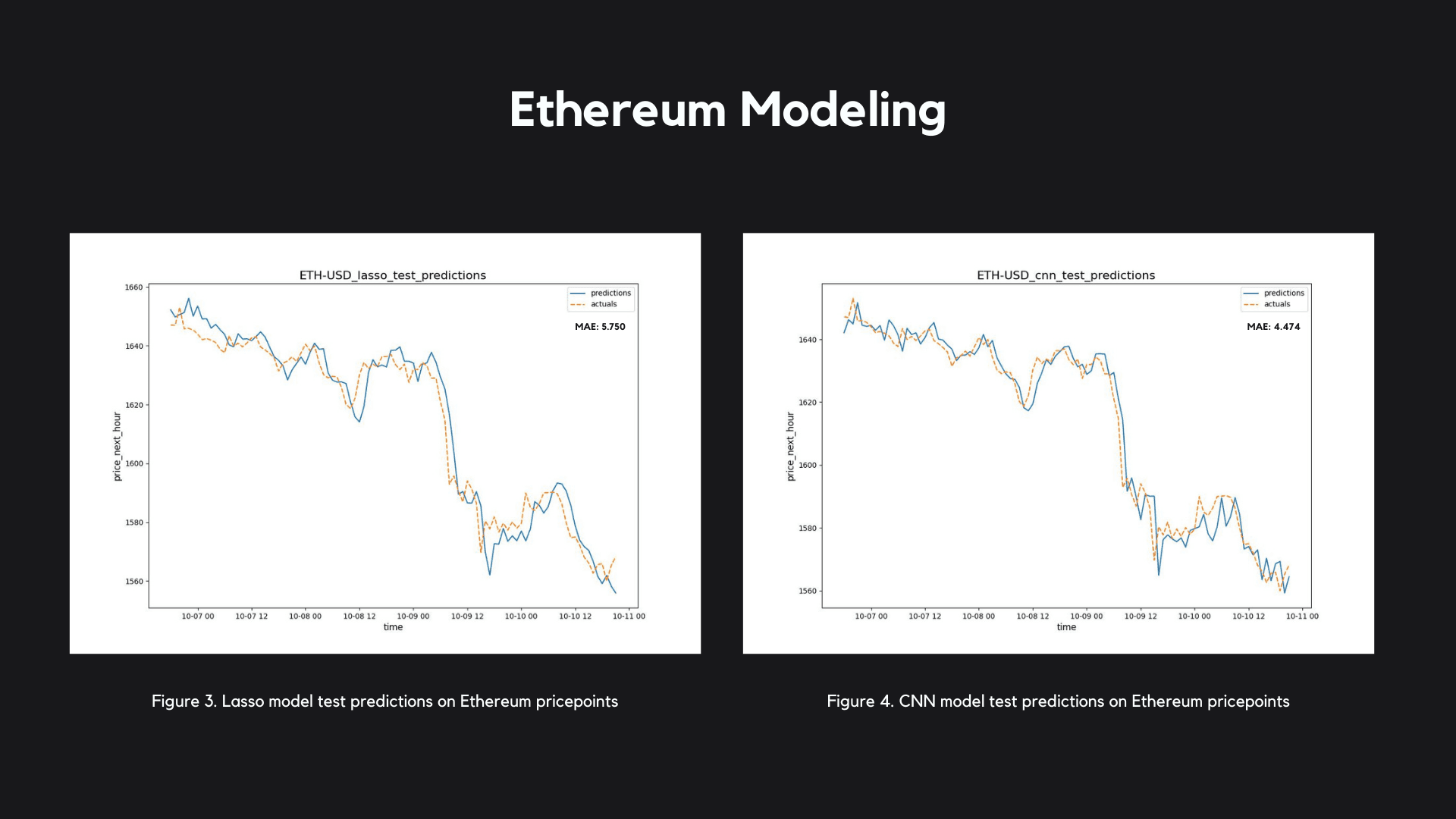
The Lasso Regressor performed extremely well for it's simplicity - it's a lightweight, efficient, and beautiful algorithm, very fast to train and easy to deploy. It garnered a mean absolute error of 88.143 on Bitcoin price predictions (fig.1) and 5.750 on Ethereum price predictions (fig.3).
I found that a Convolutional Neural Network (CNN) performed far better on both Bitcoin and Ethereum predictions compared to a Long-Short Term Memory (LSTM) Neural Network, and it's relative parameter simplicity combined with its accuracy made it a clear choice for deployment. The CNN model garnered a mean absolute error of 64.711 on Bitcoin price predictions (fig.2) and 4.474 on Ethereum price predictions (fig.4).
Modeling Recommendations
Modeling recommendations based on these experiments and used in this application can be seen below.
Machine Learning:- ✅ Lasso: fast, powerful, simple, and accurate - primary recommendation
- 🔵 LightGBM: most efficient ensemble method, most likely requires further custom feature engineering
- ✅ Convolutional Neural Network: fast, powerful, extremely lightweight, and accurate - primary recommendation
- ❌ Long Short-Term Memory Neural Network: complex, slow, and doesn't tolerate current features well; not recommended for use in current project
Prediction Service
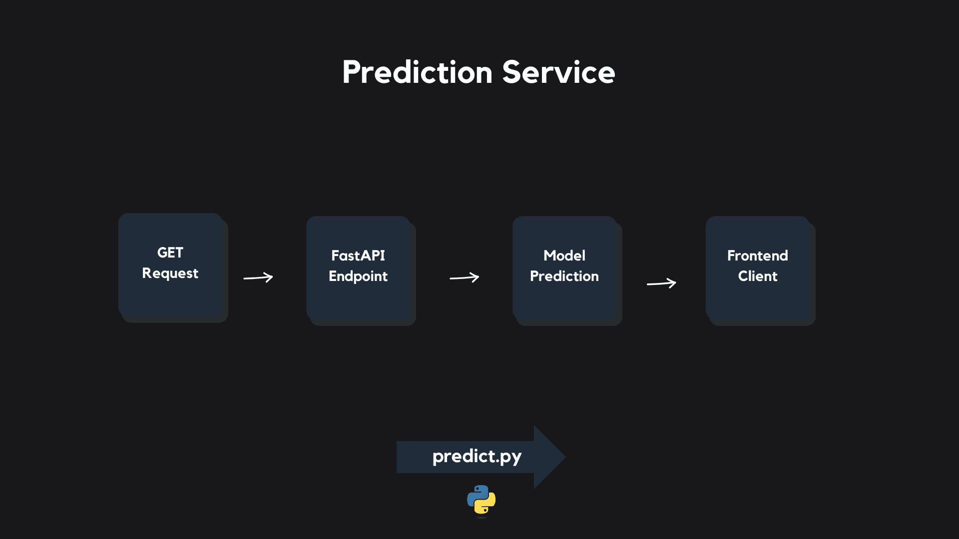
Our Prediction Service endpoint was built using FastAPI, and responds to GET requests parameterized for a cryptocurrency, timepoint, and model. The Prediction Service is containerized with Docker.
After a valid request is made, the Prediction Service loads the requested model, downloads the past 24 hours of candle data for that cryptocurrency up to and including the requested timepoint, and computes a feature vector from those datapoints.
The feature vector is passed to the loaded model and a prediction is made. The prediction is then packaged along with metadata into a PredictionResult.
Finally, the PredictionResult object is delivered to the requester for parsing.
Continuous Delivery
Our Prediction Service is deployed onto a Raspberry Pi 5, which runs using an arm64 microchip.
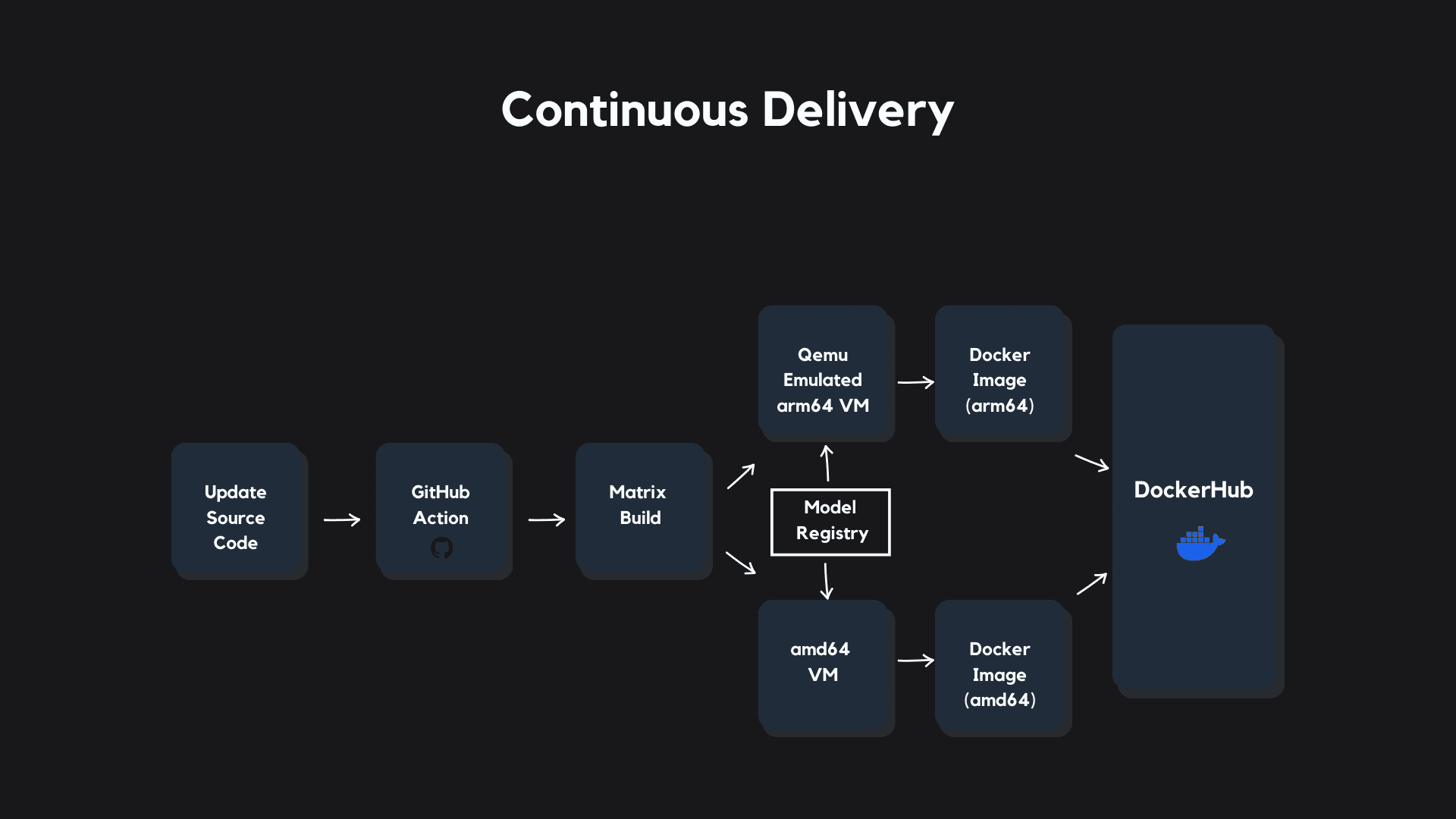
My overarching goal when designing this pipeline was to keep the Prediction Service deployable across servers using both amd64 and arm64 microchip architectures. This gives us a wide range of deployment targets down the road as requirements change, and a lot of ease in terms of deployment choices for any of the big cloud providers.
I used a matrix build triggered inside of a GitHub Action to concurrently build two separate Docker images: the first is executable on an amd64 microchip, and the second can be executed on an arm64 microchip.
When new source code passes our CI pipeline and a pull request is merged into our repository's main branch, our CD pipeline triggers a workflow that spins up two virtual machines. A simple Python script executed within the pipeline pulls our models from the model registry and downloads them into each virtual machine.
In one virtual machine, we emulate an arm64 microchip using QEMU and build the Prediction Service into a Docker image that's executable on our Raspberry Pi.
Simultaneously, on a regular GitHub Azure virtual machine (which natively uses an amd64 chip) we build the Prediction Service into a separate Docker image that's executable on amd64 microchips. This image can be used to deploy the Prediction Service to any of the standard cloud providers in a relatively straight forward way.
After each image holding our Prediction Service and models is done building, they are pushed to our Docker Hub repository, where we can easily pull them down for deployments.
Continuous Deployment
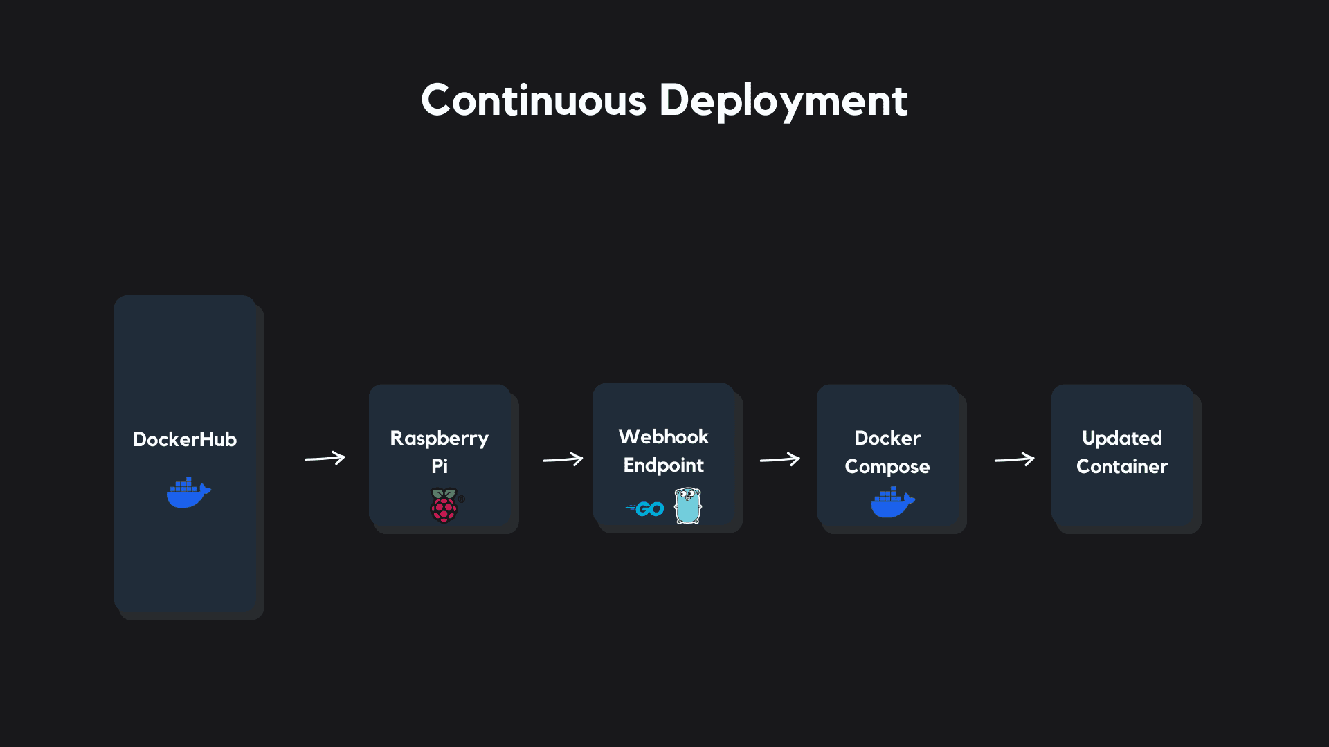
Working with a Raspberry Pi gave us a ton of control over the infrastructure and configuration choices for our server.
To tie our software supply chain together I built a custom Continuous Deployment pipeline for our Raspberry Pi that rolls out an updated container anytime a new image is pushed to our Docker Hub repository.
First, we set up a tunnel into the Raspberry Pi using Cloudflare that routes traffic from our domain into the server.
I built a simple endpoint with Golang that gets deployed onto our server along with our Prediction Service container. The endpoint listens for webhooks posted from Docker Hub whenever we push a new arm64 image to our repository.
When a POST request from Docker Hub is sent with a valid deployment key, the Golang endpoint triggers a script that pulls our new image from Docker Hub, and rolls it out on the server. We used Docker Compose to orchestrate container upgrades.
Finally, we built our tunnel, webhook endpoint, and the container into services on the Raspberry Pi, which starts them on boot and restarts them on any failures.